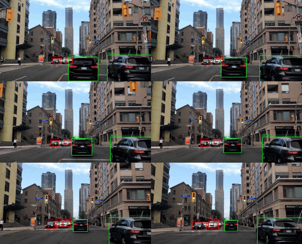
🚗 Car detection with YOLO

Hello folks! 👋 This is my first blog in github pages. I didn’t know about github pages until an amazing and greatly talented friend of mine Ramkrishna Acharya, told me about it. A big thanks to him. I wandered about and finally got with it. Someday I will definitely share about how I strolled around different sites and finally got it. Alright, now getting into the main topic, ‘Car Detection with YOLO’.

Contents

• What is object detection
  
• Detail about project
  
• Implementation
  

What is object detection?

Before we plunge into our main topic, let us first understand what image classification and localization is. Well, image classification is used to classify the type of object present in an image. It is basically related to what is in the image. Whereas, localization refers to figuring out where in the picture is the object we want to detect located. Thus, detection is image classification with localization. That’s what we’re trying to achieve here.

You know the autonomous driving system, right? It uses detection systems to detect pedestrians, trees, vehicles, traffic lights and many more that come up on the road. But here, we will only be detecting the presence of a car in the image using YOLO(You Only Look Once) algorithm. As the name suggests, this algorithm only looks once into the grid of an image. If the grid contains an object, it’ll use it otherwise it will ignore it, and only include other grids containing the objects.

Detail about project

In this tutorial, we’ll be building a Convolutional Neural Network that can detect the presence of a ‘Car’ in an image. We first need to locate the ‘car’ in the image. In general there can be multiple object in the image such as, car, pedestrian, motorcycle and background. For this, the model will return the possible object in the image out of 4 of these objects by the softmax function.

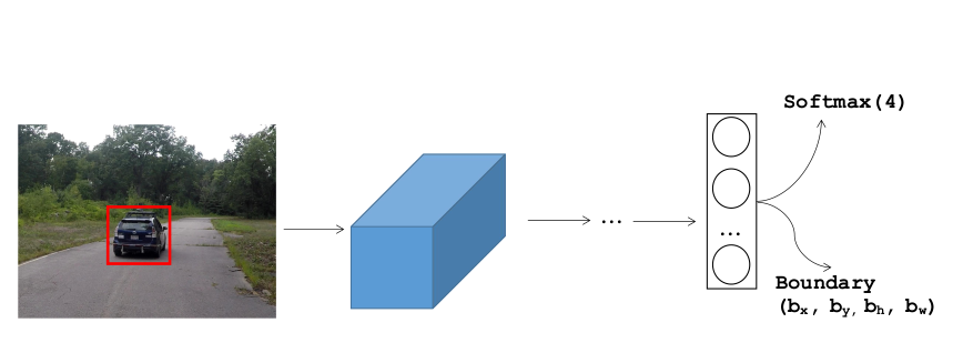
Now if we want to localize the car in the image as well, we can have the NN to output other output units, (\(b_x, b_y, b_h, b_w\)) which are dimensions of red bounding box for the detected object in the image.

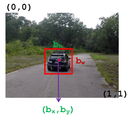
Now the algorithm outputs four parameters (\(b_x, b_y, b_h, b_w\)) as well as class labels(car, pedestrian, motorcycle, background). Therefore, for this example, the output variable will be a vector:
\(y = \left[ \begin{array}{ccc} P_{c}\\ b_{x}\\ b_{y}\\ b_{h}\\ b_{w}\\ c_{1}\\ c_{2}\\ c_{3}\\ \end{array} \right]\)
Where,
\(P_c = \left\{\begin{matrix} 1 & if\; object \\ 0 & if\; background \end{matrix}\right.\) representing the presence of object(i.e., car, pedestrian, motorcycle, background))
\(b_x, b_y\) = mid-point of an anchor box
\(b_h, b_w\) = height and width of an anchor box
\(c_1, c_2, c_3\) = class labels for car, pedestrian, motorcycle (i.e., excluding background)

There are two ways to predict the object in the image, sliding window and YOLO algorithm.

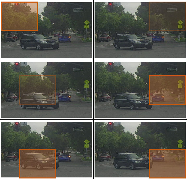
To get the bounding box for the the object in the image, we run the classifier throughout the image and try to locate the region of the object. But sliding window does not seem to perfectly take the object’s boundary in the image taking relatively more amount of CPU. On the other hand we have YOLO algorithm. It uses a popular technique called Non Maximum Suppression for drawing a boundary box around the object in the image(if present). A grid of \(s \times s\) is placed on the image. Then image classification and localization(that we just talked about) is applied to each of these grids. What YOLO does is, it takes each grid and if it does not find an object in the grid then it does not look back at that grid. But if it does, it calculates the mid-point of the image and assigns the object to that grid cell which takes the responsibility for predicting the object in the image.

Multiple grid/boxes can claim for the mid-point. Therefore, the box with the highest probability of overlapping is taken as the bounding box. So now let’s get our hands more dirty 😅 Below are the necessary details for this tutorial:

1. Input = Images each of shape \((m , 608, 608, 3)\)
2. Number of anchor boxes = 5 (to cover the 80 classes)
3. Number of grid boxes = \(19 \times 19\)
4. Output = A bounding box with recognized class. Each of these bounding box will be represented by 6 numbers (\(P_c, b_x, b_y, b_h, b_w, c\)). We’ll be covering a total of 80 classes (\(c = 80\)).

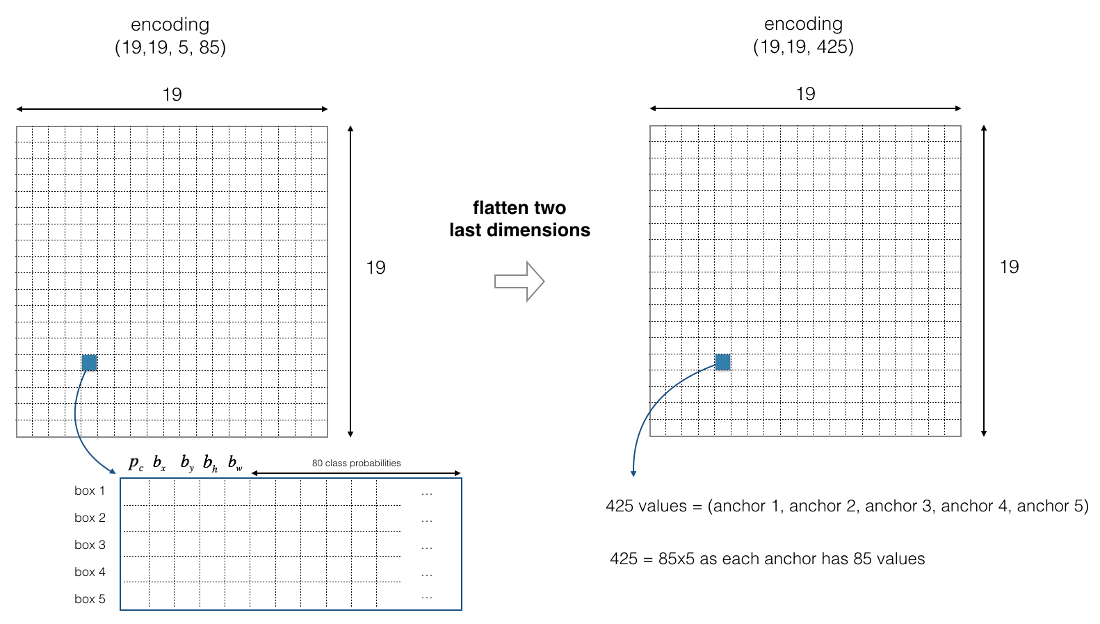
The preprocessed image of dimension \((608, 608, 3)\) is reduced by a factor of 32 into a \((19, 19, 5, 85)\). For simplicity, we’ll flatten the last two dimension of the shape (\(19, 19, 5, 85\)) to be (\(19, 19, 425\)). So in this tutorial we’ll be taking a \(19 \times 19\) grid and each cell has all the parameters(i.e., \(P_c, b_x, b_y, b_h, b_w\)).
One last thing I want you to understand before we look at the code is Class Score. The class score is calculated as: \(score_{c, i} = p_c \times c_i\), as in figure 5. Here, \(p_c\) is the probability that there is an object and \(c_i\) denotes a certain class from the list of 80 classes.

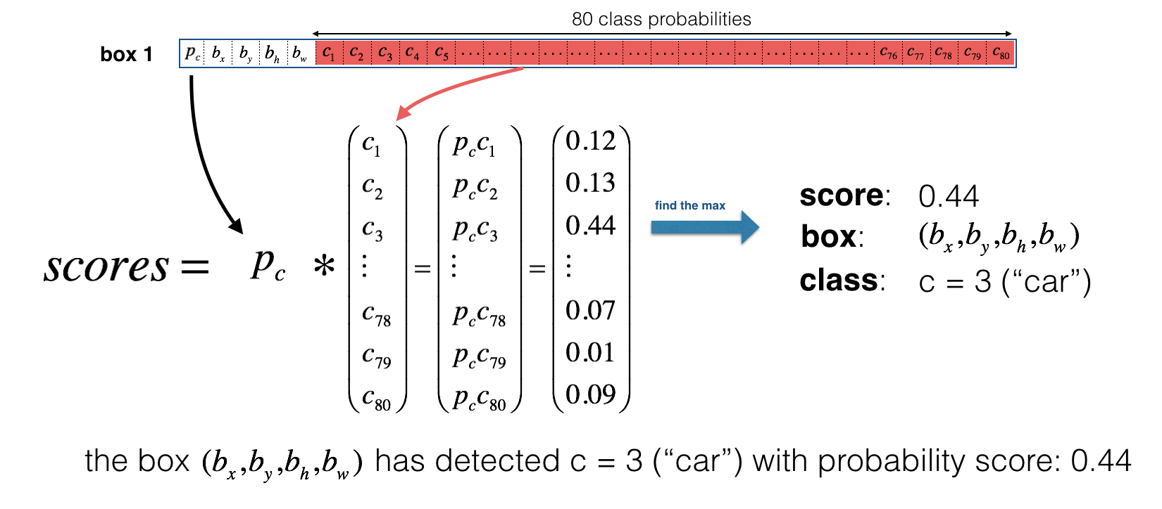
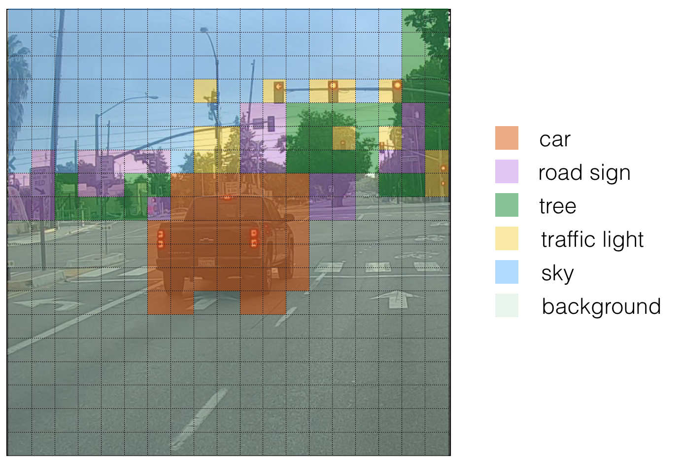
Class score is used to determine class label \(c\) for a box. For each grid box in the image, we calculate the class score and assign that box a class. So we can visualize this like in the figure below.

Implementation

Let us now start implementing it. We’ll be going step-wise. First thing’s first, let’s import all the necessary packages. Now, we’ll create a filter box to get rid of any box for which the class “score” is less than a threshold. The model gives us a total of \((19, 19, 5, 85)\) numbers, each box described by 85 different numbers. These boxes can be rearranged to the following variables:

• box-confidence: tensor of shape \((19 \times 19, 5, 1)\) containing \(p_c\) (confidence probability that there’s some object) for each of the 5 boxes predicted in each of the 19x19 cells.
• boxes:tensor of shape \((19 \times 19, 5, 4)\) containing the midpoint and dimensions \((b_x, b_y, b_h, b_w)\) for each of the 5 boxes in each cell.
• box_class_probs: tensor of shape \((19 \times 19, 5, 80)\) containing the “class probabilities” \((c_1, c_2, ... c_{80})\) for each of the 80 classes for each of the 5 boxes per cell.

We’ll create a mask using a threshold and use tensorflow to apply the mask to the variables above. Now it’s time we remove overlapping boxes. For this we’ll use Non-Max Suppression technique (as discussed above) that uses a function called “Intersection over Union”. How it’s done? We define a box using its two corners: upper left (\(x_1,y_1\)) and lower right (\(x_2,y_2\)) instead of using the midpoint, height and width. (This makes it a bit easier to calculate the intersection). After that we calculate the difference. This is to check if the boxes intersect with each other or not. We can visualize it as:

The calculated value of IoU helps to compute the overlap of the box with all other boxes, and remove boxes that overlap significantly for the condition iou >= iou_threshold. Before starting the training, one last implementational detail to implement is evaluating dimension of image. We’ll be call two methods of YOLO:

• boxes = yolo_boxes_to_corners(box_xy, box_wh) which converts the yolo box coordinates (x,y,w,h) to box corners’ coordinates (x1, y1, x2, y2) to fit the input of yolo_filter_boxes
• boxes = scale_boxes(boxes, image_shape) YOLO’s network was trained to run on 608x608 images. If you are testing this data on a different size image–for example, the car detection dataset had 720x1280 images–this step rescales the boxes so that they can be plotted on top of the original 720x1280 image.

Now, we’ll test a pre-trained model. Before training, we’re also defining number of anchor boxes and classes(as we discussed in the beginning). Finally, we can use our own image and predict it using the following function.

Credits and References

The ideas presented in this notebook came primarily from deeplearning.ai’s Convolutional Neural Network course’s assignment on Coursera . You can find the necessary files in this github repo.

Comments