🖼🖌Art generation with Neural Style Transfer

2021, Feb 22    

I love arts and paintings😍😍 and I bet you also do. I have a very close friend of mine who is a great artist. You can look at his works and contact him through facebook or linkedin(not advertising though😅😅). Well, we will also be doing something very similar to art. But we will be cunning and instead of painting one by ourself, we will be using two different images and generating an art like image. Is this possible?😂😂😂 Yes, it is. And this is probably going to be one of the most interesting post and I’m sure you’re going to love this.

So, as usual let us first understand few things. Why? Oh come on, you know “Little knowledge is dangerous.”, right? If we directly look at the code you’re going to lose yourself in the middle of nowhere and I don’t think you want to do that.😁😁

Contents

• Introduction
  
• Understanding Neural Style Transfer
  
• Mathematics behind Neural Style Transfer
  
• Implementation
  
• Credits and references
  

---

Introduction

We can have Neural Network to process text, audio, image, graph, etc. as an input. Using these organized set of data it can learn different features respective to the type of input fed to it and a final prouct is developed, known as model. This developed model maybe used for the same purpose or for a different purpose. For instance, a model developed for facial recognition maybe used for a different purpose such as, image processing task or somthing similar. Note that, the type of data the model processes hasn’t changed. You might be wondering how this is possible. This is possible because neural networks are engineered to extract the features from the fed data and these extracted features are same for data of same type(features extracted from one image out of 100 images tend to be similar). So here we will be using deep convolutional neural network to generate an art using a pretrained Deep CNN.

Understanding Neural Style Transfer

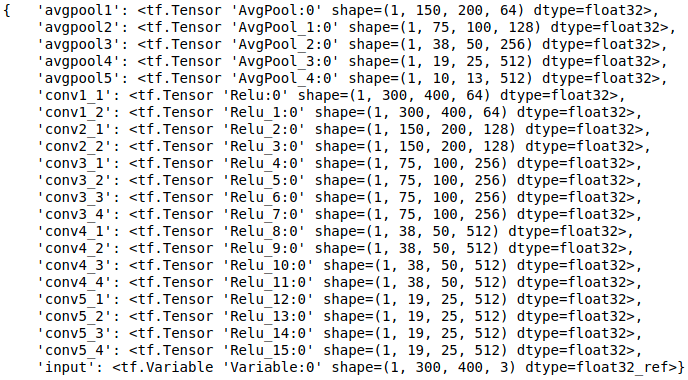
We will be using a pretrained Neural Network which is the reason of using the term ‘Neural’. The idea of using a network trained on a different task and applying it to a new task is called a transfer learning, which is exactly what we will be doing here. Therefore, Neural Style Transfer means, transferring the style from one image onto another image and generating a new image, with the combined features of both images using a pretrained Deep CNN called VGG Network. To be even more precise, we’ll be using VGG-19, a 19-layer version of the VGG network. Following is the structure of the VGG-19 model we will be using.

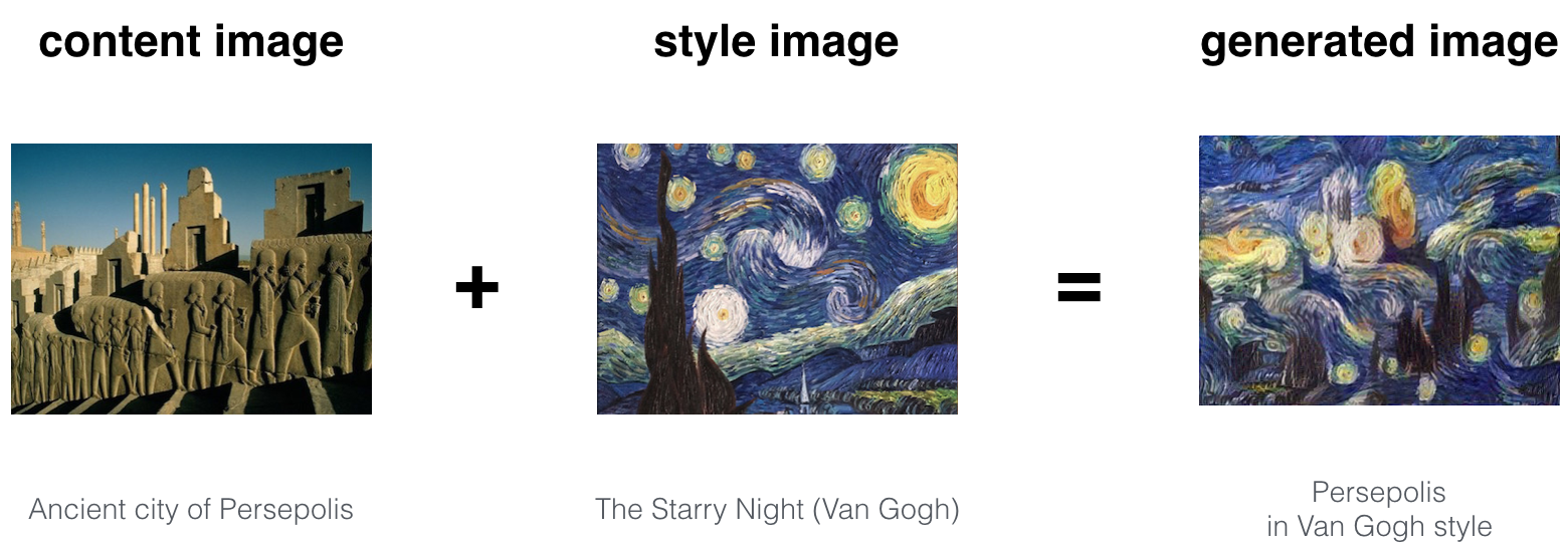
Throughout this tutorial, you will be coming across the term Contet, Style and Generated image. For our ease, we’ll be using a notation \('C'\) for Content image, \('S'\) for Style image and \('G'\) for Generated image. Content image is the image where we want to apply style of Style image and Generated image is the finally produced image.

In order to implement neural style transfer, we need to look at the features extracted by ConvNet(Convolutional Neural Network) at various layers, the shallow and the deep layer. We want no stones left unturned, that is, features at all these layers are very important to be recorded. To know what these deep ConvNets are learning,

1. Pick a unit in layer 1. Then find the \(9\) image patches that maximize the unit’s activation.
2. Repeat step 1 for layer 2, 3, 4 and so on.

In deeper layers, a hidden unit will see a larger region of the image. Where at the extreme end each pixels could hypothetically affect the output of the layers of the NN. So what does this actually mean? Let’s visualize it for \(5\; layers\) of NN.

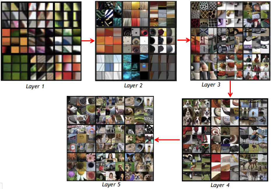
In the first layer, you can see a total of 81 boxes. In the first 9 boxes, we can find some blur textures and some lines. It’s not very clear since it’s in the beginning of the NN. These shallower networks of a ConvNet tend to detect only lower-level features of images such as edges and simple textures.

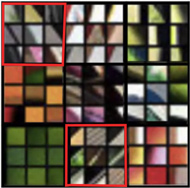
But as the network begins getting deeper and deeper they tend to detect higher-level features of images such as more complex textures as well as object classes as you can see in layers \(3\), \(4\) and \(5\).

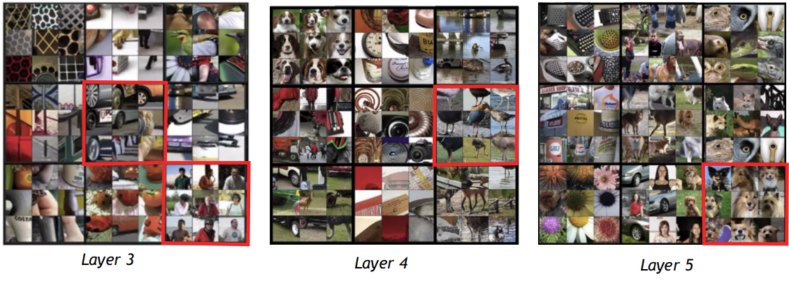
In the above figure 4, in layer 3, the blury image has now become clearer, and more complex objects. Objects such as Car’s wheel, human faces can easily be seen. Similarly in layer 4 and layer 5. There are \((9\times9)\) image patches having clear dog’s images, bird’s legs, etc. which is focusing on particulars.

Mathematics behind Neural Style Transfer

Hope so we are good so far. Until now, we’ve seen what actually deep ConvNets are learning. Now let us see how we improve over the image patches inorder to get a better results. What do you think I might be talking about?🤔🤔 So when it comes to making result better, it’s definitely the gradient descent and cost function. Let’s see the algorithm.

1. Find the generated image \(G\).
2. Initialize the generated image \(G\) randomly(say \(100\times100\times3\)).
3. Define the cost function \(J(G)\).
4. Use gradient descent to minimize \(J(G)\)
   \(G = G - \frac{\alpha J(G)}{\alpha G}\)
   We are actually updating the pixel values of the image \(G\)

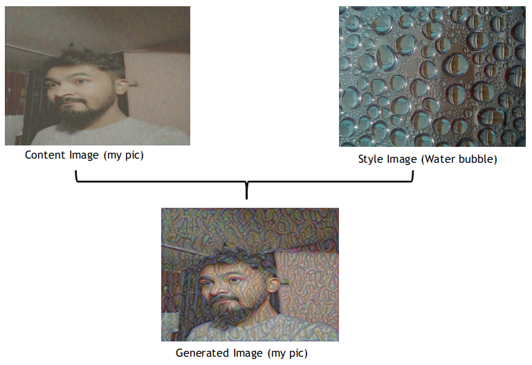
There’s no worries in step 1 and 2. It’s step 3 and 4 that we actually need to workon. The reason why we calculate the cost function is to find the similarity between the (Content image, Generated image) and (Style image, Generated image). Below is my image, before applying Water Bubble style and the generated image after apply the style. This is a sample of what we’ll be doing in this blog.

Alright, the overall cost function can be defined as:
\(J(G) = \alpha J_{content}(C, G) + \beta J_{style}(S, G)\)
Let us see how can calculate Content cost function \(J_{content}(C, G)\) and Style cost function \(J_{style}(S, G)\).

Content Cost function

Let \(a^{[l][C]}\) and \(a^{[l][G]}\) be the activation for a hidden layer \(l\) of the VGG-19 Network. The cost function is then calculated as: \(J_{content}(C, G) = \frac{1}{4\times n_{H}\times n_{W}\times n_{C}} \sum_{all\;entries}^{}(a^{C} - a^{G})^{2}\)

Style Cost Function

Before looking at the style cost function, we need to understand about the \(style \; matrix\). The image we pass through Deep CNN is convolved into a matrix of dimension \((n_H \times n_W \times n_C)\). These images have different channels. Each of these channels have differing activations produced while processing by the Deep CNN. The \('style'\) of an image means how correlated are the activations across these channels.

Here you can see 5 different color channels. But in practice, there can be lot more channels than what we can see here. So what does it mean for these two channels being highly correlated or uncorrelated?

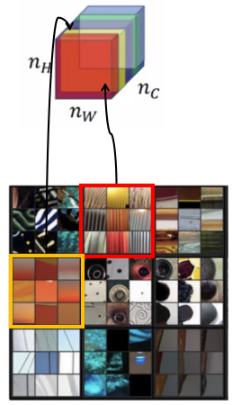
Well, if the \(Red\) and \(Yellow\) channels are highly correlated, then vertical textures produced by the \(Red\) channel tend to have orangish tint(texture produced by the \(yellow\) channel). And it’s just the contrary when these two channels are uncorrelated, i.e., the vertical textures don’t tend to have orangish tint. So these textures tells us that which of these high level texture components tend to occur often or don’t occur often or occur together or don’t occur together in part of a generated image. Let the activation for layer \(l\) be denoted by \(a^{[l]}_{i,j,k}\) = activation at (i, j, k),
where,
\(i\) = Height, \(j\) = Width and \(k\) = Channels
The style matrix \(G^{l}\) is of dimension \(n^{l}_{C} \times n^{l}_{C}\) and it is calculated by:

1. For style image: \(G^{l(S)}_{kk^{'}} = \sum_{i=1}^{n^{l}_{H}} \sum_{j=1}^{n^{l}_{W}}(a_{ijk}^{[l](S)} * a_{ijk^{'}}^{[l](S)})\)
2. Similarly, for generated image: \(G^{l(G)}_{kk^{'}} = \sum_{i=1}^{n^{l}_{H}} \sum_{j=1}^{n^{l}_{W}}(a_{ijk}^{[l](G)} * a_{ijk^{'}}^{[l](G)})\)

Style matrix is also called gram matrix. Gram matrix \(G\) of a set of vectors \((v_{1}, v_{2}, ..., v_{n})\) is the matrix of dot products, whose entries are: \(G_{ij} = v_{i}^{T}.v_{j} = np.dot(v_{i}, v_{j})\).
So having this much, we can now calculate the style cost function as:
\(J_{style}^{[l]}(S, G) = \left \| G^{[l](S)} - G^{[l](G)} \right \|^{2}\)
\(or, J_{style}^{[l]}(S, G) = \frac{1}{(2n_{H}^{l}n_{W}^{l}n_{C}{l})^{2}} \sum_{k}\sum_{k^{'}}(G^{l(S)}_{kk^{'}} - G^{l(G)}_{kk^{'}})^{2}\)
\(or, J_{style}^{[l]}(S, G) = \frac{1}{4\times n_{C}^{2}\times(n_{H}\times n_{W})^{2}} \sum_{i=1}^{n_{C}} \sum_{j=1}^{n_{C}} (G_{(gram)i,j}^{(S)} - G_{(gram)i,j}^{(G)})^{2}\)
\(J_{style}^{[l]}(S, G) = \sum_{l} \lambda^{l} J_{style}^{[l]}(S, G)\)
Where, \(\lambda^{l}\) refers to weight to be assigned for different layers during training.

Before beginning the implementation, one more thing I would like to include here is about \(unrolling\). We will be using it in the implementation so it’s necessary for us to understand what is. Below is an illustration:

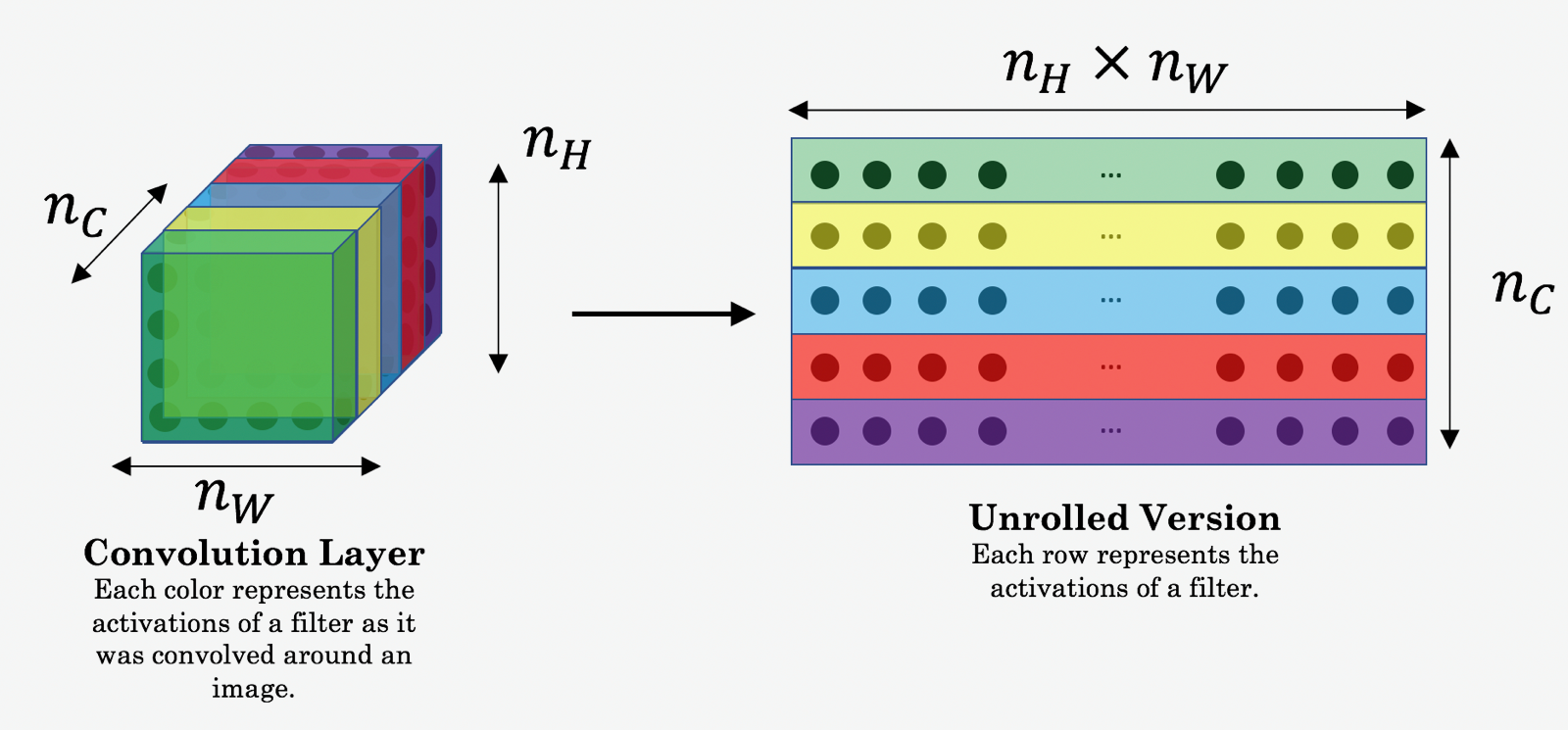
Basically, what’s happening here is, we want to change the shape from \((m,n_{H}, n_{W}, n_{C})\) to \((m, n_{H}\times n_{W}, n_{C})\) and for this we’ll be using two tensorflow methods, <div style="font-family: courier new; color: crimson; background-color: #f1f1f1; padding: 2px; font-size: 105%; border: 1px solid black; padding: 2px; text-align: left;"> tf.reshape( tensor, shape, name=None ) </div>

Implementation

You’ve reached here, this means, you’re so much eager and curious about neural style transfer’s implementation. Great!!🎊🎉🎊✊✊ Now let’s move on with the implementation. Here we will be doing exactly what we’ve just discussed above but programmatically.

Importing package

Let’s begin with some important package imports.

Style image and Content image

Also let’s initialize variables with our content image and style images.

Generated image

Now we initialize the “generated_image” asa noisy image from the loaded content image. By initializing the pixels of the generated image to be mostly noise but slightly correlated with the content image, this will help the content of the “generated” image more rapidly match the content of the “content” image.

Loading pre-trained model

As already mentioned, in this tutorial we will be using a pre-trained VGG-19 model. You can download the model from here with license.

Computing content cost

Now we compute the content cost.

Computing style cost

Before computing style cost, if you remember, we must compute gram matrix, right? So let us first compute gram matrix. Now in order to make it easier, let us first compute style cost for a single layer. And we will be calling this function over and over again for other hidden units. Then finally, you can see below how we’re going to use the above function to compute the overall style cost for a style image. Also note, since we need to assign the weights to different neuron of different layer for pre-trained model, we will first assign the value of \(\lambda^{l}\)(weights).

Computing total cost

So as per our step followed above, it’s time we compute the total cost by summing up the Content cost and Style cost.

Content, Style and total cost

To get the program to compute the content cost, we will now assign a_C and a_G to be the appropriate hidden layer activations. We will use layer conv4_2 to compute the content cost. The code below does the following:

1. Assign the content image to be the input to the VGG model.
2. Set a_C to be the tensor giving the hidden layer activation for layer “conv4_2”.
3. Set a_G to be the tensor giving the hidden layer activation for the same layer.
4. Compute the content cost using a_C and a_G.

Optimizer

We will be using Adam Optimizer to reduce the cost J.

Model implementation

Finally we implement the model.

Run the following command to generate the an artistic image. Be careful while copying the code about the files and folders location.

You’ll find your images saved in the folder ‘Output’(according to this program). Congratulations, we have finally generated an image using a Neural Style Transfer on a pre-trained ConvNet. You can find necessary files and this assignment’s notebook in this Github repo.

Credits and references

This whole work is a part of Coursera’s deeplearning.ai course: Convolutional Neural Network’s Week 4’s course and assignment. Other references are:

• Leon A. Gatys, Alexander S. Ecker, Matthias Bethge, (2015). A Neural Algorithm of Artistic Style
• Harish Narayanan, Convolutional neural networks for artistic style transfer.
• Log0, TensorFlow Implementation of “A Neural Algorithm of Artistic Style”.
• Karen Simonyan and Andrew Zisserman (2015). Very deep convolutional networks for large-scale image recognition
• MatConvNet.

Comments