Image Compression and Color Quantization using K-Means Clustering

🤔🤔 Do you remember taking a selfie and trying out different filters on your photos, getting so excited to upload it to facebook or insta? 😁😁😁 If you have then you must have seen the filter’s effect come into action but if I’m not wrong, you probably have no idea how it’s happening behind the scene, do you? Well if you have the idea, that’s good but if you don’t have then that’s double good. Why? Because this blog will give you an insight of what’s it really like applying a filter to an image and how it’s really happening.

Contents

• Introduction
  
• Concept
  
• Installation
  
• Implementation
  

Introduction

What we will be doing is, compress an image of higher size relatively into a smaller size. By size I mean image’s memory consumption, not the aspect ratio (though it is also somewhat related to the size 😅). Before we begin, let’s familiarize ourselves with what Image Compression, Color Quantization and K-Means Clustering is.

Concept

Basically, K-Means Clustering is used to find the central value (centroid) for k clusters of data. Then each data point is assigned to the cluster whose center is nearest to \(k\). Then, a new centroid is calculated for each of the k clusters based upon the data points that are assigned in that cluster. In our case, the data points will be Image pixels. Assuming that you know what pixels are, these pixels actually comprises of 3 channels, Red, Green and Blue. Each of these channels’ have intensity ranging from 0 to 255, i.e., altogether 256 values. So as a whole, the total number of colors in each pixel is, \(256 \times 256 \times 256\). Each pixel(color) has \(2^{8}\) colors acquiring 8 bits of memory. Thus, each pixel requires \(8+8+8\), i.e., 24 bits of memory for storage.

Now, using K-Means clustering, we’ll try to group pixels of similar color together in \(k\) clusters, i.e., 8 different colors. Instead of each pixel originally representing \(256 \times 256 \times 256\) colors, each pixel can only represent 8 possible colors. The most surprising thing is, each pixel now requires only \(3\)(\(2^{3}\) = 8) bits of memory, instead of original 24 bits. Here in the process, we’re breaking all possible colors of the RGB color space over k colors. This is called Color Quantization and during this, the k centroids of the clusters are representative of 3 dimensional RGB color space. It will now replace the colors of all points in their cluster and thus the image will only have k colors in it.

Installation

This was a little bit of a concept for understanding, what we are going to do. 😁 Let us now begin with our real task. Throughout this tutorial, we’ll be using some of OpenCV and Python libraries. Basically, we’ll use Scikit-learn, Matlplotlib and Numpy.

Let’s install some dependencies(I assume you have anaconda installed).

1. Installing OpenCV
   • conda install -c conda-forge opencv

</div>

1. Installing Scikit-learn
   • conda install -c conda-forge scikit-learn

</div>

1. Installing a python 2D plotting library, i.e., matplotlib
   • conda conda install -c conda-forge matplotlib

</div>

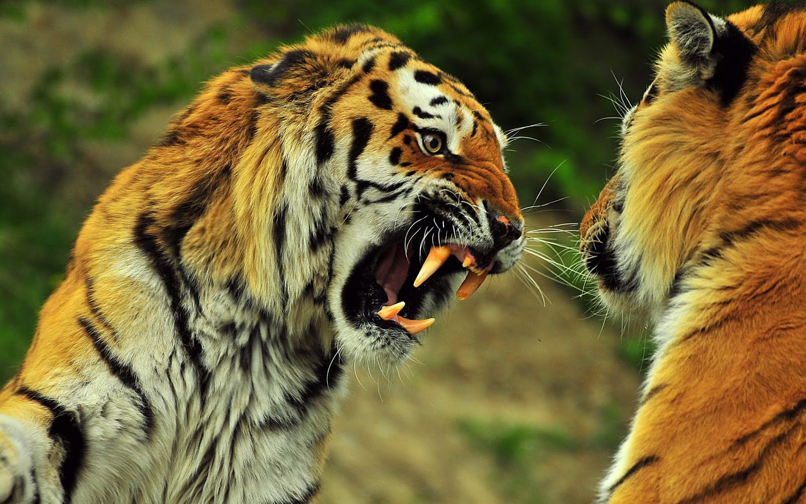
For this tutorial, you can download below image from here.

Implementation

It’s time to get our hands dirty. Let us first assign the downloaded image to a variable.

Note: In case the url may not work, you'll need to manually download the file and give the link to that image file. For example, you can simply do the following after you've downloaded the file (in my case, it is in 'images' folder).

Moving on, let’s import some important modules. First let’s see features of original file size of the image that we just downloaded (in KB) and run the code. You’ll see the output as below:

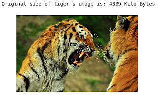
Now we’ll use numpy and K-Means clustering from Sklearn as for transforming the dimension of image. In order to transform the image into certain dimension, we first need to extract the number of rows and columns of the image above. After that, we’ll reshape the image into a dimension compatible with the original shape of the above image. We’ll see something like the one in the image below when executed in the Jupyter Notebook.

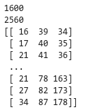
It’s the dimension of the image and the pixels that we just reshaped into a matrix of dimension \((numberOfRows \times numberOfCols) \times 3\). Here, \(numberOfRows = 2560\) and \(numberOfCols = 1600\).

Now time for some magic. This may take sometime to execute. You will find the output to be as follow.

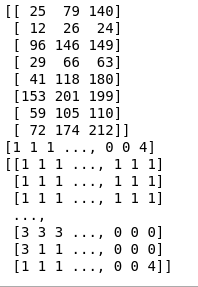
This is the final matrix of cluster_centroids and labels. Now we iteratively assign the clustered_centroids into our initialized matrix.

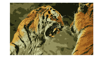
We can also see the difference (the background, color of tiger’s fur, etc.) in the original and the compressed image of the tiger that we just produced. Now one last final thing to do, i.e., see the change in size of compressed_tiger.jpg'

Bamm! We’ve successfully compressed the tiger’s image by 60%. And this is indeed a great compression. You can further change the value of n_cluster to see the variations.

Credits

The work presented in this notebook came primarily from IBM’s coursera course Introduction to Computer Vision with Watson and OpenCV

Comments